import numpy as np
import matplotlib.pyplot as plt
%matplotlib inline
What is machine learning ?
When we need Machine Learning
When the business logic is too complicated to be directly coded like for voice recognition, or logic is hidden like for customer behaviour on website, machine learning can be used to find this mysterious business logic.

How it “learn” ?
First we select a mathematics model parametrable like a polynom or a decision tree. Then an optimizer will compare output given by model and output expected, it will tun parameters to minimize this error.

How many machine learning exist
Many! There are two kinds :
- classifier: according to input, it will try to select an category as output. Ex: try to find if customer will buy someting, sort cat images, etc
- regression: according to input, it will try to predict values. Ex: all forecast purpose, …

How to represent business to learn ?
Represent a whole dataset to be visualize quickly, is complicated with real user case. Can you quick see a classifier dataset when you look a huge table full of numbers ?
But if you chose machine learning such as input is a position and output is a color. Then each prediction becomes a pixel and the whole dataset an image.

def classifier_business(x, y):
    if x<0.2 and y > 0.3:
        return (0.9, 0.1, 0.1)
    if x > 0.6:
        return (0.1, 0.9, 0.1)
    return (0.1, 0.1, 0.9)
def regression_business(x, y):
    return (x + y) / 2, (1- x + y) / 2, (2 - x + y) / 2
def business_to_dataset(size, mapping):
    # Apply mapping over all pixel grid
    dataset = np.empty((size, size, 3))
    space = np.linspace(0, 1, size)
    for x in range(0, size):
        for y in range(size-1, -1, -1):
            dataset[y, x] = mapping(space[x], 1-space[y])
    return dataset
def print_dataset(datasets, titles=''):
    # Print image if there are only one image
    if type(datasets) != list:
        fig, ax = plt.subplots(figsize=(6, 6))
        ax.imshow(datasets)
        ax.set_title(titles)
        ax.set_xticklabels(['-0.2', '0', '0.2', '0.4', '0.6', '0.8', '1'])
        ax.set_yticklabels(['1.2', '1', '0.8', '0.6', '0.4', '0.2', '0'])

    # Pring images if there are many images
    else:
        size = len(datasets)
        fig, axis = plt.subplots(ncols=size, figsize=(6*size, 6))
        for (ax, dataset, t) in zip(axis, datasets, titles):
            ax.imshow(dataset)
            ax.set_title(t)
            ax.set_xticklabels(['-0.2', '0', '0.2', '0.4', '0.6', '0.8', '1'])
            ax.set_yticklabels(['1.2', '1', '0.8', '0.6', '0.4', '0.2', '0'])

    plt.show()
classifier_dataset = business_to_dataset(500, classifier_business)
regression_dataset = business_to_dataset(500, regression_business)
print_dataset([classifier_dataset, regression_dataset], ['Classifier business', 'Regression Business'])
Clipping input data to the valid range for imshow with RGB data ([0..1] for floats or [0..255] for integers).
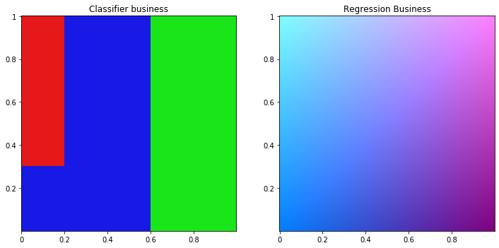
This our dataset, the mysterous logic we have to find. Classifier at left, regression at right.
def pick_pixels(dataset, number):
    index = np.random.randint(0, 500, size=(number, 2))
    space = np.linspace(0, 1, 500)

    pixels = dataset[index[:, 1], index[:, 0]]
    xy = np.array([[space[x], space[y]] for x, y in index])
    return xy.astype('float'), pixels
def apply_ml(ml, dataset, size=200):
    xy, pixels = pick_pixels(dataset, size)
    ml.fit(xy, pixels)

    X,Y = np.mgrid[0:1:0.002, 0:1:0.002]
    xy = np.vstack((X.flatten(), Y.flatten())).T
    return ml.predict(xy).reshape(500, 500, 3).transpose(1, 0, 2)
def discretize_dataset(i):
    return np.round(i * 100).astype('int')
Classifier
from sklearn.tree import DecisionTreeClassifier

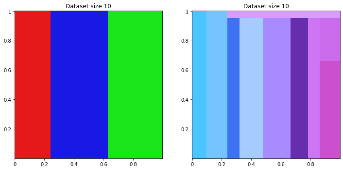
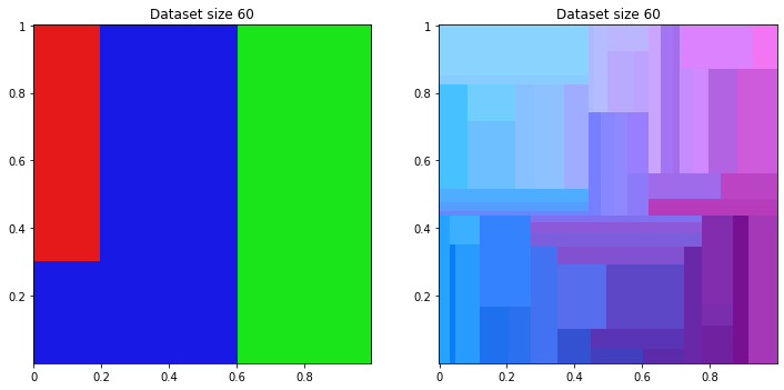
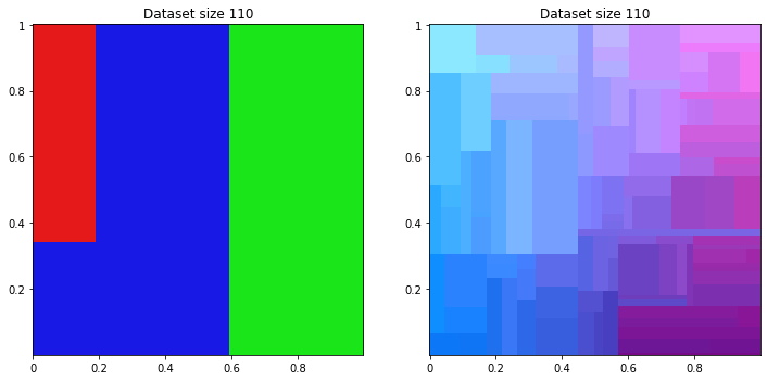
for size in range(10, 200, 50):
    class_class_dataset = apply_ml(DecisionTreeClassifier(), discretize_dataset(classifier_dataset), size) / 100
    class_reg_dataset   = apply_ml(DecisionTreeClassifier(), discretize_dataset(regression_dataset), size) / 100
    title = 'Dataset size {}'.format(size)
    print_dataset([class_class_dataset, class_reg_dataset], [title, title])
Clipping input data to the valid range for imshow with RGB data ([0..1] for floats or [0..255] for integers).
Clipping input data to the valid range for imshow with RGB data ([0..1] for floats or [0..255] for integers).
Clipping input data to the valid range for imshow with RGB data ([0..1] for floats or [0..255] for integers).
Clipping input data to the valid range for imshow with RGB data ([0..1] for floats or [0..255] for integers).
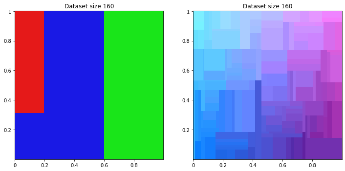
Of course on classifier dataset, classifier machine learning sucess to find logic. For regression dataset, it split domain in many squares to fill gradient.
Regression
from sklearn.linear_model import LinearRegression

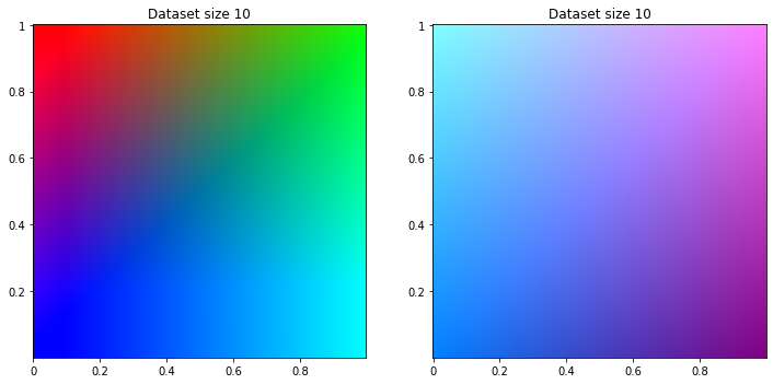
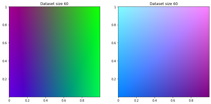
for size in range(10, 200, 50):
    reg_class_dataset = apply_ml(LinearRegression(), classifier_dataset, size)
    reg_reg_dataset   = apply_ml(LinearRegression(), regression_dataset, size)
    title = 'Dataset size {}'.format(size)
    print_dataset([reg_class_dataset, reg_reg_dataset], [title, title])
Clipping input data to the valid range for imshow with RGB data ([0..1] for floats or [0..255] for integers).
Clipping input data to the valid range for imshow with RGB data ([0..1] for floats or [0..255] for integers).
Clipping input data to the valid range for imshow with RGB data ([0..1] for floats or [0..255] for integers).
Clipping input data to the valid range for imshow with RGB data ([0..1] for floats or [0..255] for integers).
Clipping input data to the valid range for imshow with RGB data ([0..1] for floats or [0..255] for integers).
Clipping input data to the valid range for imshow with RGB data ([0..1] for floats or [0..255] for integers).
Clipping input data to the valid range for imshow with RGB data ([0..1] for floats or [0..255] for integers).
Clipping input data to the valid range for imshow with RGB data ([0..1] for floats or [0..255] for integers).

And of course too, on regression dataset, regression machine learning success to find logic. For classifier dataset, engine tries to separate color but gradient remains.
Neuronal Network
import tensorflow as tf


Build network
def build_nn(size, discretize=False):
    deep = [tf.keras.layers.Dense(l,  activation=tf.nn.tanh, use_bias=True) for l in size]

    nn = tf.keras.models.Sequential(
        [tf.keras.layers.Dense(2,  activation=tf.nn.tanh, use_bias=True)]
        + deep +
        [tf.keras.layers.Dense(3,  activation=tf.nn.sigmoid, use_bias=False)])
    loss = 'categorical_crossentropy' if discretize else 'mean_squared_error'
    nn.compile(optimizer='adam', loss=loss)
    return nn
More tuned
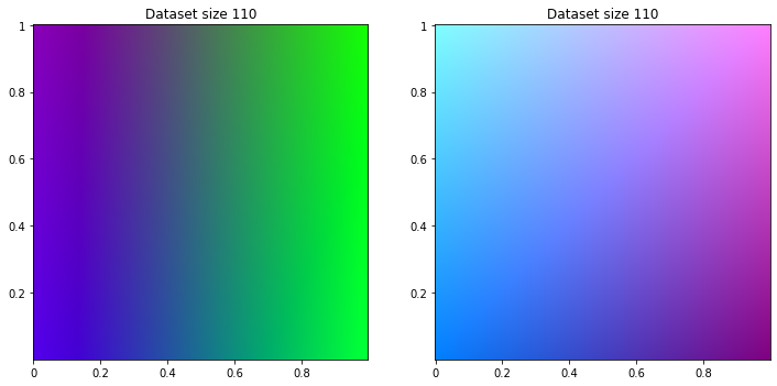
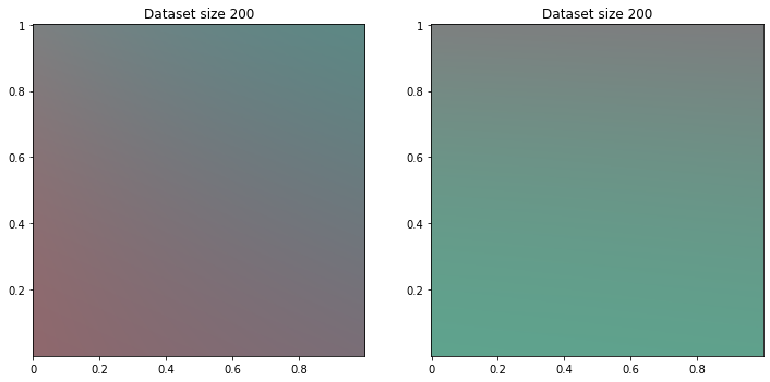
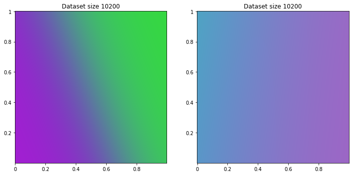
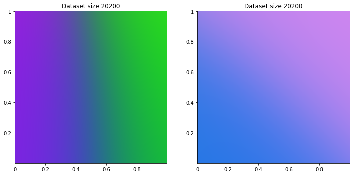
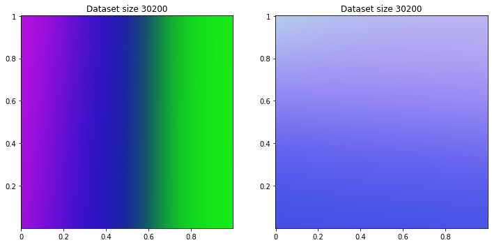
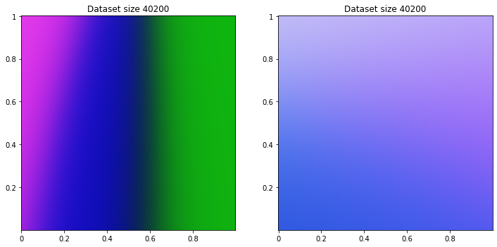
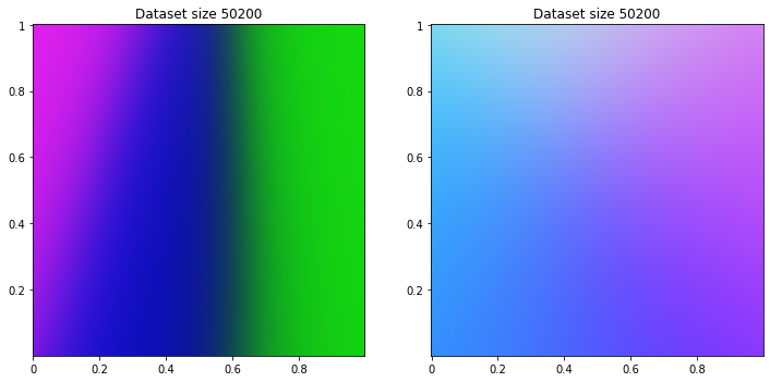
for size in range(200, 60000, 10000):
    nn_class_dataset = apply_ml(build_nn([5, 5], True), classifier_dataset, size)
    nn_reg_dataset = apply_ml(build_nn([5, 5]), regression_dataset, size)
    title = 'Dataset size {}'.format(size)
    print_dataset([nn_class_dataset, nn_reg_dataset], [title, title])
200/200 [==============================] - 0s 921us/sample - loss: 1.1965
200/200 [==============================] - 0s 384us/sample - loss: 0.1267
10200/10200 [==============================] - 0s 36us/sample - loss: 1.1012
10200/10200 [==============================] - 0s 32us/sample - loss: 0.0870
20200/20200 [==============================] - 1s 36us/sample - loss: 1.0935
20200/20200 [==============================] - 1s 27us/sample - loss: 0.0498
30200/30200 [==============================] - 1s 35us/sample - loss: 0.9780
30200/30200 [==============================] - 1s 27us/sample - loss: 0.0416
40200/40200 [==============================] - 1s 30us/sample - loss: 0.9120
40200/40200 [==============================] - 1s 28us/sample - loss: 0.0379
50200/50200 [==============================] - 1s 28us/sample - loss: 0.9611
50200/50200 [==============================] - 2s 31us/sample - loss: 0.0329
Benchmark with true business
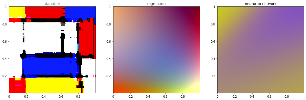
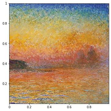
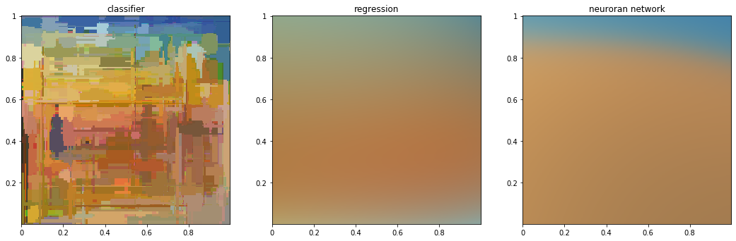
Now we can apply engines on more complicated dataset. As we use image to see data, I will use artwork.
from PIL import Image
from sklearn.ensemble import RandomForestClassifier
from sklearn.linear_model import Ridge
from sklearn.preprocessing import PolynomialFeatures
from sklearn.pipeline import make_pipeline
Monet
monet = np.asarray(Image.open('resources/monet.jpg')) / 256

class_monet_dataset = apply_ml(RandomForestClassifier(n_jobs=4), discretize_dataset(monet)) / 100
reg_monet_dataset = apply_ml(make_pipeline(PolynomialFeatures(degree=5), Ridge()), monet)
nn_monet_dataset = apply_ml(build_nn([5, 7, 4]), monet, 50000)

print_dataset(monet)

print_dataset([class_monet_dataset, reg_monet_dataset, nn_monet_dataset], ['classifier', 'regression', 'neuroran network'])
/home/jolainfra/perso/machin-learning-course/venv/lib/python3.6/site-packages/sklearn/ensemble/forest.py:245: FutureWarning: The default value of n_estimators will change from 10 in version 0.20 to 100 in 0.22.
  "10 in version 0.20 to 100 in 0.22.", FutureWarning)


50000/50000 [==============================] - 2s 31us/sample - loss: 0.0192
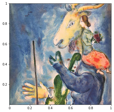
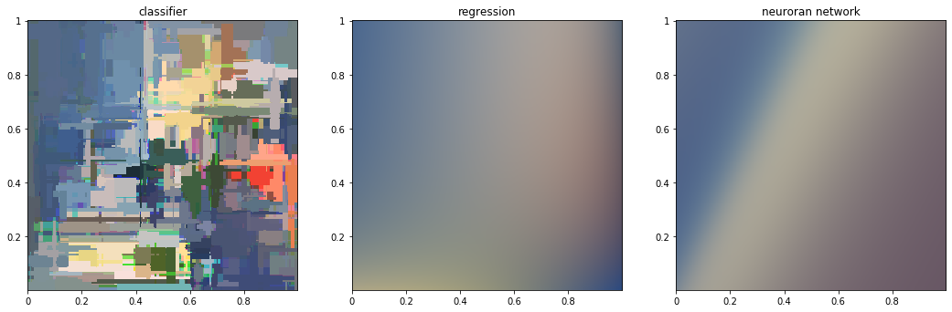
Chagall
chagall = np.asarray(Image.open('resources/chagall.jpg')) / 256

class_chagall = apply_ml(RandomForestClassifier(n_jobs=4), discretize_dataset(chagall)) / 100
reg_chagall = apply_ml(make_pipeline(PolynomialFeatures(degree=8), Ridge()), chagall)
nn_chagall = apply_ml(build_nn([8, 8, 4]), chagall, 50000)

print_dataset(chagall)

print_dataset([class_chagall, reg_chagall, nn_chagall], ['classifier', 'regression', 'neuroran network'])
/home/jolainfra/perso/machin-learning-course/venv/lib/python3.6/site-packages/sklearn/ensemble/forest.py:245: FutureWarning: The default value of n_estimators will change from 10 in version 0.20 to 100 in 0.22.
  "10 in version 0.20 to 100 in 0.22.", FutureWarning)


50000/50000 [==============================] - 1s 27us/sample - loss: 0.0298
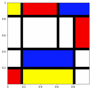
Mondrian
mondrian = np.asarray(Image.open('resources/mondrian.jpg')) / 256

class_mondrian = apply_ml(RandomForestClassifier(n_jobs=4), discretize_dataset(mondrian)) / 100
reg_mondrian = apply_ml(make_pipeline(PolynomialFeatures(degree=5), Ridge()), mondrian)
nn_mondrian = apply_ml(build_nn([5, 7, 4], True), mondrian, 50000)

print_dataset(mondrian)

print_dataset([class_mondrian, reg_mondrian, nn_mondrian], ['classifier', 'regression', 'neuroran network'])
/home/jolainfra/perso/machin-learning-course/venv/lib/python3.6/site-packages/sklearn/ensemble/forest.py:245: FutureWarning: The default value of n_estimators will change from 10 in version 0.20 to 100 in 0.22.
  "10 in version 0.20 to 100 in 0.22.", FutureWarning)


50000/50000 [==============================] - 2s 35us/sample - loss: 1.8750
WARNING: Logging before flag parsing goes to stderr.
W0628 12:43:12.497635 140184450438976 image.py:693] Clipping input data to the valid range for imshow with RGB data ([0..1] for floats or [0..255] for integers).